Recurrent Neural Network
Table of Contents
- 1. Introduction
- 2. Training by Gradient descent
- 3. Training by Global optimization methods
- 4. Limitations of RNN
- 5. Architectures
- 5.1. Fully recurrent
- 5.2. Elman networks and Jordan networks
- 5.3. Hopfield
- 5.4. Echo state
- 5.5. Independently RNN (IndRNN)
- 5.6. Recursive
- 5.7. Neural history compressor
- 5.8. Second order RNNs
- 5.9. Long short-term memory
- 5.10. Gated recurrent unit
- 5.11. Bi-directional
- 5.12. Continuous-time
- 5.13. Hierarchical
- 5.14. Recurrent multilayer perceptron network
- 5.15. Multiple timescales model
- 5.16. Neural Turing machines
- 5.17. Differentiable neural computer
- 5.18. Neural network pushdown automata
- 5.19. Memristive Networks
- 6. Applications
- 7. Page Dumps & Lecture Notes
1. Introduction
RNNs are network specifically for Sequence Modeling.
Consider a single feed forward network, it takes input and gives output at a single timestep. Lets call this the recurrent cell and use it as building block to accept sequence of input (i.e. input/output at timestep)
- We can pass inputs from multiple timesteps, but what we need is to connect the current input to input from previous timesteps
- This means we need to propagate prior computation/information through time: via. Recurrence Relation
- We do this through, Internal Memory or State: \(h_t\)
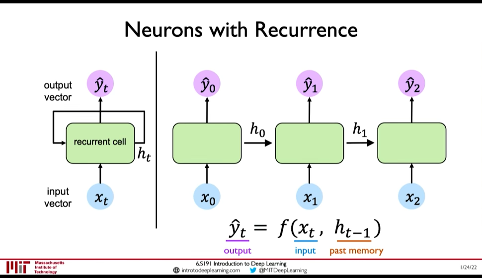
Figure 1: Recurrent NN
- In RNN, we apply a recurrence relation at every time step to process a sequence
- RNNs have a state, \(h\), that is updated at each time step as a sequence is processed
- \(h_t = f_W(x_t, h_{t-1})\) where the weight \(W\) is same across timesteps but the input \(x_t\) and the memory \(h_t\) change
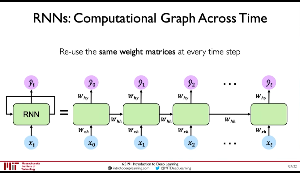
Figure 2: RNN: Computation Graph Across Time
- \(y_t = f(W_{hy}, h_t)\) why not xt ?
- \(h_t = f(W_{hh}, h_{t-1}, W_{hx}, x_t)\)
1.1. RNN can Exhibit Temporal Dynamic Bheviour
A recurrent neural network (RNN) is a class of artificial neural networks where connections between nodes form a directed graph along a temporal sequence. This allows it to exhibit temporal dynamic behavior. Derived from feedforward neural networks, RNNs can use their internal state (memory) to process variable length sequences of inputs. This makes them applicable to tasks such as unsegmented, connected handwriting recognition or speech recognition.
1.2. Finite Impulse and Infinite Impulse Networks
The term “recurrent neural network” is used indiscriminately to refer to two broad classes of networks with a similar general structure, where
- one is finite impulse: that can be unrolled and replaced with a strictly feedforward neural network
- the other is infinite impulse: a directed cyclic graph that can not be unrolled
1.3. RNN can have Memory Stored States (LSTMs, GRUs)
Both finite impulse and infinite impulse recurrent networks can have additional stored states, and the storage can be under direct control by the neural network. The storage can also be replaced by another network or graph, if that incorporates time delays or has feedback loops. Such controlled states are referred to as gated state or gated memory, and are part of long short-term memory networks (LSTMs) and gated recurrent units. This is also called Feedback Neural Network (FNN).
2. Training by Gradient descent
Gradient descent is a first-order iterative optimization algorithm for finding the minimum of a function.
2.1. BackProagation Through Time (BPTT)
The standard method is called “backpropagation through time” or BPTT, and is a generalization of back-propagation for feed-forward networks.
2.2. Real-Time Recurrent Learning (RTRL)
A more computationally expensive online variant is called “Real-Time Recurrent Learning” or RTRL, which is an instance of automatic differentiation in the forward accumulation mode with stacked tangent vectors. Unlike BPTT, this algorithm is local in time but not local in space.
In this context, local in space means that a unit's weight vector can be updated using only information stored in the connected units and the unit itself such that update complexity of a single unit is linear in the dimensionality of the weight vector. Local in time means that the updates take place continually (online) and depend only on the most recent time step rather than on multiple time steps within a given time horizon as in BPTT. Biological Neural Networks appear to be local with respect to both time and space.
2.3. LSTM for Vanishing gradient problem
2.4. Causal Recursive BackPropagation (CRBP)
The on-line algorithm called causal recursive backpropagation (CRBP), implements and combines BPTT and RTRL paradigms for locally recurrent networks.[77] It works with the most general locally recurrent networks.
3. Training by Global optimization methods
Training the weights in a neural network can be modeled as a non-linear global optimization problem.
The most common global optimization method for training RNNs is genetic algorithms, especially in unstructured networks.
Other global (and/or evolutionary) optimization techniques may be used to seek a good set of weights, such as simulated annealing or particle swarm optimization.
4. Limitations of RNN
RNN as presented above have the following limitations:
- Encoding Bottleneck: RNN need to take long sequence of information and condense it into a fixed representation
- Slow, no parallelization
- Not long memory: ~10, 100 length sequences are ok with LSTM, but not ~1000
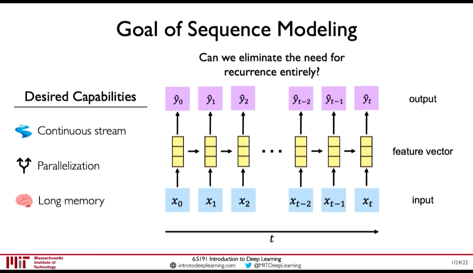
Figure 3: Desired Capabilities of RNN @ 0:41:48
In contrast to those limitations, what we want is:
- Continuous Stream
- Parallelization
- Long Memory
Idea 1: Feed everything into dense network: (@ 0:42:52)
- Recurrence is eliminated, but
- Not scalable
- No order
- No long memory
Idea 2: Identify and Attend to what's important (@ 0:42:58)
5. Architectures
5.1. Fully recurrent
Basic RNNs are a network of neuron-like nodes organized into successive layers. Each node in a given layer is connected with a directed (one-way) connection to every other node in the next successive layer.[ citation needed ] Each node (neuron) has a time-varying real-valued activation. Each connection (synapse) has a modifiable real-valued weight.
For supervised learning in discrete time settings, sequences of real-valued input vectors arrive at the input nodes, one vector at a time. At any given time step, each non-input unit computes its current activation (result) as a nonlinear function of the weighted sum of the activations of all units that connect to it. Supervisor-given target activations can be supplied for some output units at certain time steps. For example, if the input sequence is a speech signal corresponding to a spoken digit, the final target output at the end of the sequence may be a label classifying the digit.
In reinforcement learning settings, no teacher provides target signals. Instead, a fitness function or reward function is occasionally used to evaluate the RNN's performance, which influences its input stream through output units connected to actuators that affect the environment. This might be used to play a game in which progress is measured with the number of points won.
Each sequence produces an error as the sum of the deviations of all target signals from the corresponding activations computed by the network. For a training set of numerous sequences, the total error is the sum of the errors of all individual sequences.
5.2. Elman networks and Jordan networks
5.3. Hopfield
The Hopfield network is an RNN in which all connections are symmetric. It requires stationary inputs and is thus not a general RNN, as it does not process sequences of patterns. It guarantees that it will converge. If the connections are trained using Hebbian learning then the Hopfield network can perform as robustcontent-addressable memory, resistant to connection alteration.
5.4. Echo state
5.5. Independently RNN (IndRNN)
5.6. Recursive
A recursive neural network[32] is created by applying the same set of weights recursively over a differentiable graph-like structure by traversing the structure in topological order. Such networks are typically also trained by the reverse mode of automatic differentiation.[33][34] They can process distributed representations of structure, such as logical terms. A special case of recursive neural networks is the RNN whose structure corresponds to a linear chain. Recursive neural networks have been applied to natural language processing.[35] The Recursive Neural Tensor Network uses a tensor-based composition function for all nodes in the tree.[36]
5.7. Neural history compressor
5.8. Second order RNNs
5.9. Long short-term memory
Long short-term memory (LSTM) is a deep learning system that avoids the vanishing gradient problem. LSTM is normally augmented by recurrent gates called “forget gates”.[42] LSTM prevents backpropagated errors from vanishing or exploding.[39] Instead, errors can flow backwards through unlimited numbers of virtual layers unfolded in space. That is, LSTM can learn tasks
[12]
that require memories of events that happened thousands or even millions of discrete time steps earlier. Problem-specific LSTM-like topologies can be evolved.[43] LSTM works even given long delays between significant events and can handle signals that mix low and high frequency components.
Many applications use stacks of LSTM RNNs[44] and train them by Connectionist Temporal Classification (CTC)[45] to find an RNN weight matrix that maximizes the probability of the label sequences in a training set, given the corresponding input sequences. CTC achieves both alignment and recognition
5.10. Gated recurrent unit
5.11. Bi-directional
5.12. Continuous-time
A continuous time recurrent neural network (CTRNN) uses a system of ordinary differential equations to model the effects on a neuron of the incoming spike train.
CTRNNs have been applied to evolutionary robotics where they have been used to address vision,[53] co-operation,[54] and minimal cognitive behaviour.[55]
5.13. Hierarchical
5.14. Recurrent multilayer perceptron network
5.15. Multiple timescales model
5.16. Neural Turing machines
Neural Turing machines (NTMs) are a method of extending recurrent neural networks by coupling them to external memory resources which they can interact with by attentional processes. The combined system is analogous to a Turing machine or Von Neumann architecture but is differentiable end-to-end, allowing it to be efficiently trained with gradient descent.[61]
5.17. Differentiable neural computer
Differentiable neural computers (DNCs) are an extension of Neural Turing machines, allowing for usage of fuzzy amounts of each memory address and a record of chronology.
5.18. Neural network pushdown automata
5.19. Memristive Networks
6. Applications
Applications of Recurrent Neural Networks include:
- Machine Translation
- Robot control
- Time series prediction
- Speech recognition
- Speech synthesis
- Time series anomaly detection
- Rhythm learning
- Music composition
- Grammar learning
- Handwriting recognition
- Human action recognition
- Protein Homology Detection
- Predicting subcellular localization of proteins
- Several prediction tasks in the area of business process management
- Prediction in medical care pathways